BOLD-PETCO2 CVR Data Analysis Tutorial

Introduction

The aim of this practical is to provide an overview of model-based analysis of cerebrovascular reactivity (CVR) data.

In theory, Quantiphyse can be used in combination with a variety of different MR acquisition/analysis schemes for CVR assessment. Nevertheless, with this initial version, only Blood Oxygen Level Dependent (BOLD) data can be analysed within Quantiphyse. In the coming months, we plan to optimise this aspect and add additional modelling options. At this stage, any feedback would be extremely useful, so please contact us if you would like to suggest any alteration (joana.pinto@eng.ox.ac.uk, martin.craig@nottingham.ac.uk).

Additionally, we would like to thank Dr Sana Suri for providing the example data for this tutorial and Prof Daniel Bulte for helping with the analysis pipeline.

Start the program by typing quantiphyse at a command prompt or clicking on the Quantiphyse icon  in the menu or dock.

Load the data

First, we need to load the data. For this tutorial, we will use BOLD data acquired with a simultaneous multi-slice acquisition scheme (SMS) (TR = 0.8s). We already pre-processed this data using FSL’s FEAT (brain extraction and creation of brain mask, temporal filtering (90s) and spatial smoothing (5mm)). In the future, we plan to include this initial step in Quantiphyse.

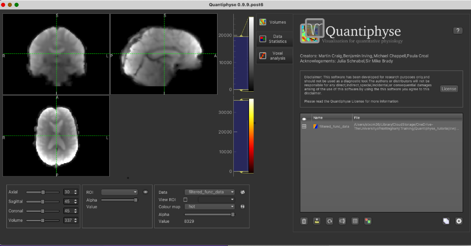
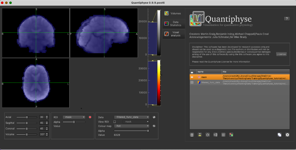
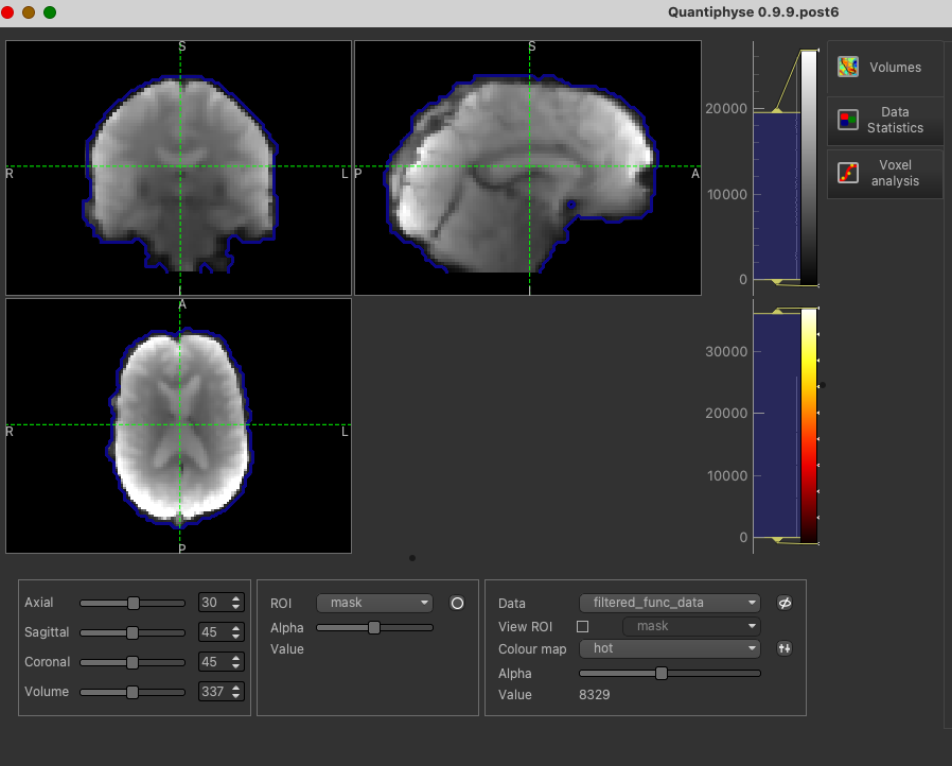
The pre-processed BOLD data is named filtered_func_data.nii.gz and the brain mask (our ROI) is mask.nii.gz. You can load these either using the menu item File->Load data or by dragging and dropping the data files into the viewer window from the file manager. If you are taking part in an organised practical workshop, the data required will be available in your home directory, in the course_data/cvr/001/cvr.feat folder.

Be sure to specify the CVR BOLD data as Data and mask file as ROI.

Filtered functional data:

With mask loaded:

When viewing the output of modelling, it may be clearer if the ROI is displayed as an outline rather than a shaded region. To do this, click on the icon to the right of the ROI selector (below the image view):

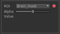
The icon cycles between display modes for the ROI: shaded (with variable transparency selected by the slider below), shaded and outlined, just outlined, or no display at all.

Note

If you accidentally load an ROI data set as Data, you can set it to be an ROI using the Volumes widget (visible by default). Just click on the data set in the list and click the Toggle ROI button.

Image view

The left part of the window normally contains three orthogonal views of your data. In this case the data is a 2D slice so Quantiphyse has maximised the relevant viewing window. If you double click on the view it returns to the standard of three orthogonal views - this can be used with 3D data to look at just one of the slice windows at a time.

• Left mouse click to select a point of focus using the crosshairs
• Left mouse click and drag to pan the view
• Right mouse click and drag to zoom
• Mouse wheel to move through the slices
• Double click to ‘maximise’ a view, or to return to the triple view from the maximised view.

View and navigation controls

Just below the viewer these controls allow you to move the point of focus and also change the view parameters for the current ROI and overlay.

Widgets

The right hand side of the window contains ‘widgets’ - tools for analysing and processing data. Three are visible at startup:

• Volumes provides an overview of the data sets you have loaded
• Data statistics displays summary statistics for data set
• Voxel analysis displays timeseries and overlay data at the point of focus

Select a widget by clicking on its tab, just to the right of the image viewer.

More widgets can be found in the Widgets menu at the top of the window. The tutorial will tell you when you need to open a new widget.

For a slightly more detailed introduction, see the Getting Started section of the User Guide.

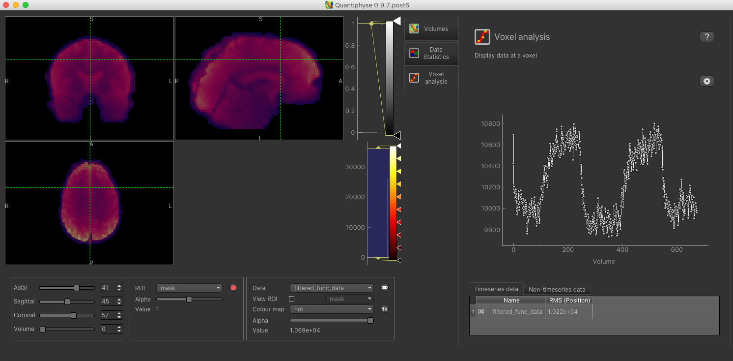
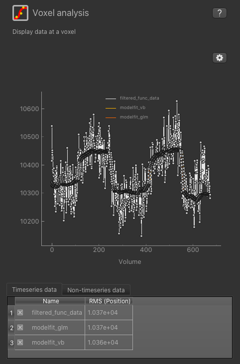
It is always helpful to check the timeseries of the BOLD-MRI data by clicking on the Voxel analysis Widget:

The practical CVR BOLD dataset follows a boxcar paradigm with alternating 60 s periods of air and hypercapnia. The voxelwise time-course clearly shows the increase in the BOLD signal during the hypercapnia blocks.

The CVR analysis Widget

This can be found under Widgets->CVR->CVR PETCO2

Acquisition Parameters

Firstly, we will select the pre-processed BOLD data and the brain mask, previously loaded. The BOLD data you loaded will probably already be selected as ‘BOLD timeseries data’ - if not select it using the list box. For the ROI, make sure you have selected the analysis mask loaded previously. It is important to make sure you have selected a suitable mask as the ROI - otherwise the analysis will be performed on every voxel in the entire volume which will be extremely slow!

Set the TR to match the dataset (0.8s):

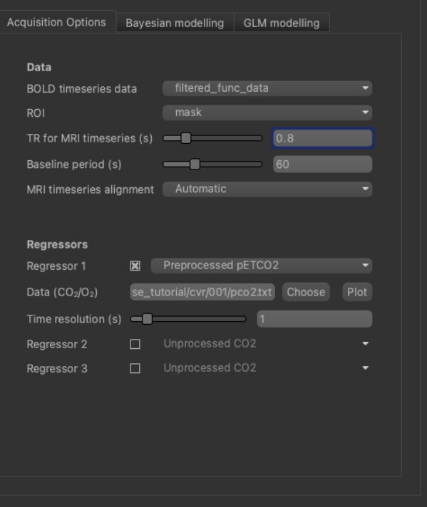
In this example, we acquired the corresponding pCO2 trace (a surrogate of CO2 arterial content) using a capnograph (this is highly encouraged). The sequence of values recorded is stored in a file named pco2.txt. This should be selected as the ‘Physiological Data’ input, either by dragging and dropping the file onto the box, or by clicking the ‘Choose’ button and selecting the file.

After loading the co2.txt file, we can click the Plot button to view a simple plot of the timeseries:

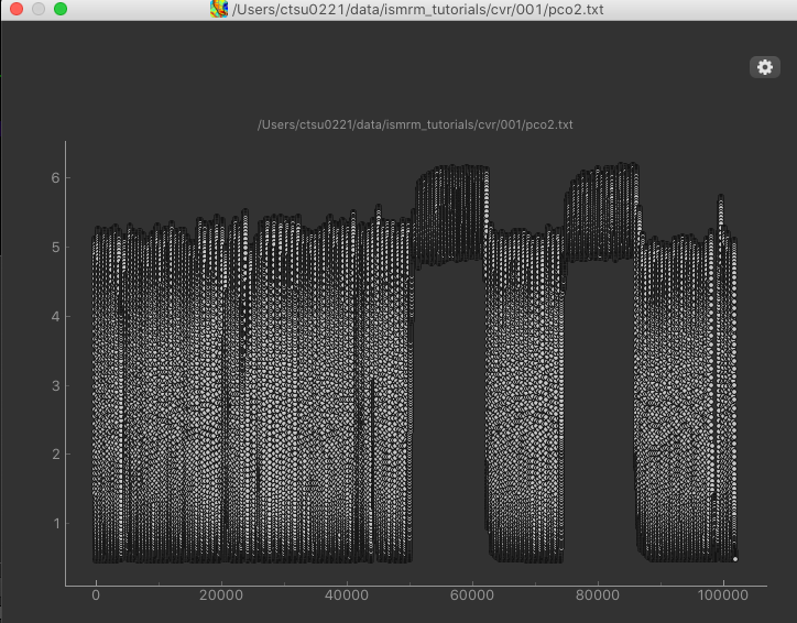
The rapid oscillations in the timeseries are caused by the subjects breathing, however we can clearly see an extended baseline period, followed by the two alternations of air and hypercapnia.

To process the PetCO2 timecourse we need some additional acquisition parameters.

• pCO2 sampling frequency: This is the number of readings of pCO2 per second
• TR: This is the TR of the BOLD data in seconds
• Baseline period: Time in seconds after the start of BOLD data acquisition, but before any manipulation of pCO2. This period is used to determine the respiratory rate and identify the end-tidal pCO2 from the CO2 timeseries

For this tutorial dataset the corresponding values are: sampling frequency = 100Hz, TR = 0.8s and baseline period = 60s.

It is also necessary to match the BOLD and PetCO2 time courses temporally. This is required because the start of the pCO2 time series does not correspond to the acquisition time of the first BOLD volume. Quantiphyse has two options for this step: manual or automatic. If you know the exact delay value (how long after the pCO2 trace started the first BOLD volume was acquired), this can be added manually. If not, by using the automatic option, Quantiphyse performs an initial cross correlation between the two timecourses to estimate the ROI (mask) average time shift. All subsequent delays obtained in the next steps will be relative to this initial one.

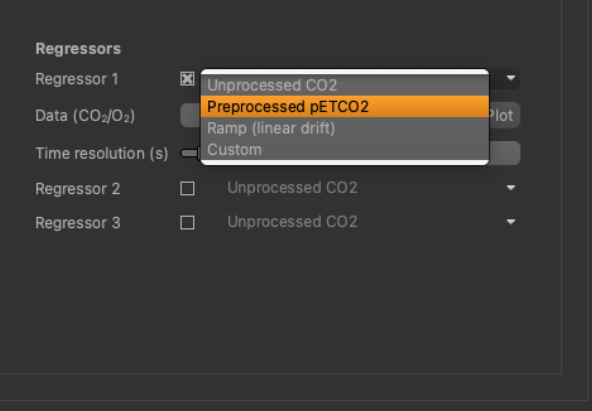
In the future, we plan to introduce more regressor options.

Modelling

Quantiphyse also allows some flexibility in terms of model fitting. Two different modelling strategies are implemented: Bayesian Inference and General Linear Modelling (GLM) approach. The former allows computation of voxelwise CVR amplitude and timing information in a single step. The GLM approach can also allow CVR timing estimation, but this step will be based on performing multiple GLM’s and selecting the best fit for each voxel.

The Bayesian modelling tool performs inference using a fast variational Bayes technique to return maps of CVR, estimated delay time (if selected).

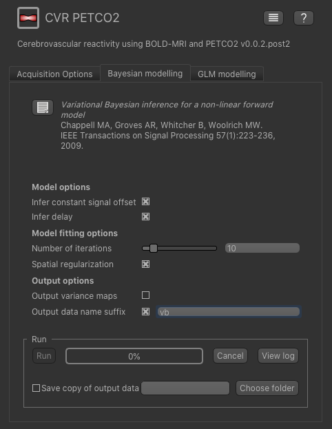
We will leave all the settings at their defaults, however to avoid the output getting confused with subsequent runs you can specify a data set name suffix - e.g. vb as above.

Choose a folder, if you would like to save a copy of the output data.

Click ‘Run’ to perform the analysis. The following output files will be generated:

• cvr_vb - The CVR map
• delay_vb - The delay time map in seconds
• sig0_vb - The constant signal offset
• modelfit_vb - The model fit

The GLM modelling tool performs a similar analysis by inverting a linear model. In order to estimate the delay time, the GLM must be fitted for a range of delay times with the best fit (least squares) selected as the output. The minimum and maximum delay times to be tested can be specified, as well as the step length. Of course, the more delay times you test the longer the analysis will take. Unlike the Bayesian approach, only the specific delay times tested will be returned in the delay time map, so this will effectively be a discrete rather than a continuous map.

In this tutorial we will tell the GLM modelling tool to search delay times between -50s and 50s, in steps of 1s, as follows:

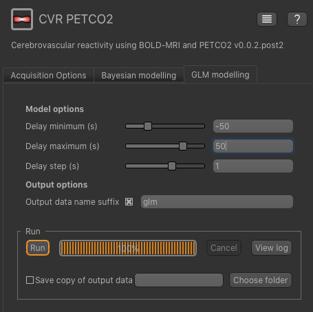
Again, you can specify an output dataset name suffix, e.g. glm.

Choose a folder, if you would like to save a copy of the output data.

Click ‘Run’ to perform the analysis. The output files will match those generated by the VB modelling, i.e. cvr_glm, delay_glm, sig0_glm and modelfit_glm

Output

To check the model fit, we can use the Voxel Analysis widget and click on voxels in the image to see the data overlaid with the model prediction.

We can also use the viewer windows to switch between the output data sets from the VB and GLM methods and compare the results.

The CVR amplitude are mostly similar, as expected. Only a few voxels around the borders tend to have higher values with the Bayesian approach.

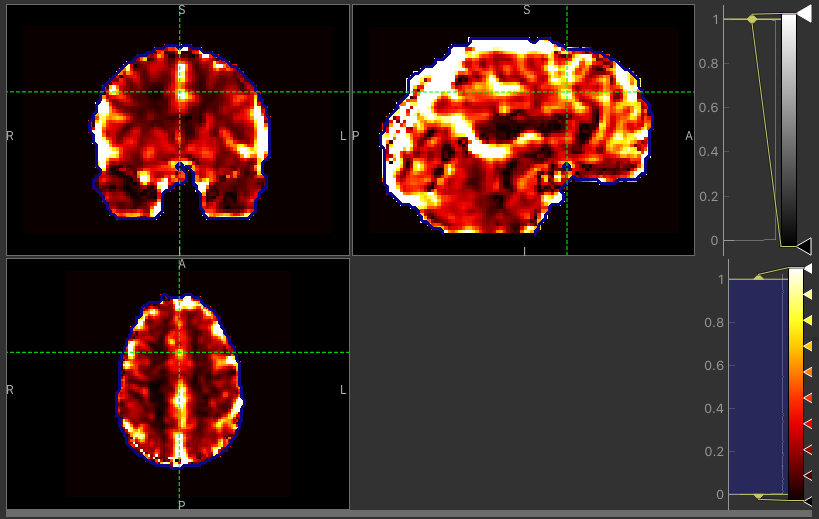
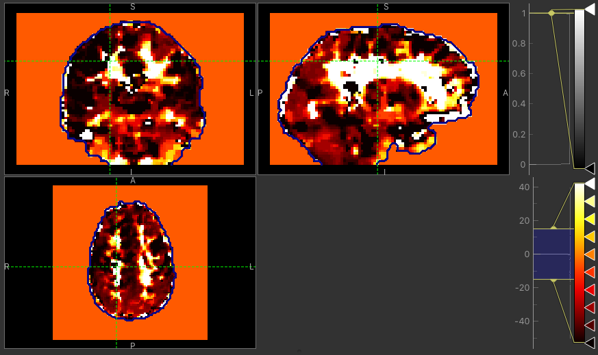
CVR map using VB

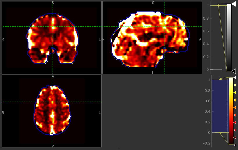
CVR map using GLM

The major difference between approaches is the delay maps. In regions with high CVR amplitude, both methods agree on the delay (mostly GM). However, in regions with lower CVR amplitude values, the Bayesian approach uses the prior and selects a delay close to the average value obtained by the automatic timeseries alignment. In contrast, the GLM selects the ‘best’ delay even when it might be extreme (e.g. in CSF).

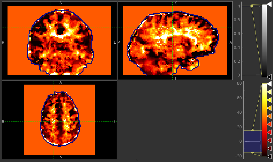
Delay map using VB

Delay map using GLM