qBOLD Tutorial
Introduction
The aim of this practical is to provide an overview of Bayesian model-based analysis [1] of Quantitative BOLD, or qBOLD, data. We will work with healthy human data [2] to quantify the reversible transverse relaxation rate (\(R_2^\prime\)), the oxygen extraction fraction (OEF) and the deoxygenated blood volume (DBV).
This data was acquired using a GESEPI ASE (Gradient Echo Slice Excitation Profile Imaging Asymmetric Spin Echo) pulse sequence [3], which deals with the three major confounding effects of qBOLD:
- Cerebral Spinal Fluid (CSF) signal contamination
- Macroscopic magnetic field inhomogeneity
- Underlying transverse T2 signal decay.
However, there are several other ways to acquire qBOLD data including standard ASE [4] and the GESSE (Gradient Echo Sampling of Spin Echo) pulse sequence [5]. This tool might also be useful for analysing data from these techniques if the aforementioned confounds can be removed in pre-processing, although this has not been tested.
Basic Orientation
Before we do any data modelling, this is a quick orientation guide to Quantiphyse if you’ve not used it before. You can skip this section if you already know how the program works.
Start the program by typing quantiphyse at a command prompt, or clicking on the Quantiphyse
icon ![]() in the menu or dock.
in the menu or dock.
Loading some qBOLD Data
If you are taking part in an organized practical workshop, the data required may be available in your home
directory, in the course_data/qbold folder.
Note
If the data is not provided, it can be can be downloaded from the Oxford
Research Archive site: https://doi.org/10.5287/bodleian:E24JbXQwO
(Click the link streamlined-qBOLD_stud… to download a compressed archive of the data).
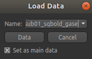
Start by loading the qBOLD data into Quantiphyse - use File->Load Data or drag and drop to load the file
sub-01_sqbold_gase.nii.gz in the sub-01/func folder. In the Load Data dialog select Data.
The data should appear as follows:
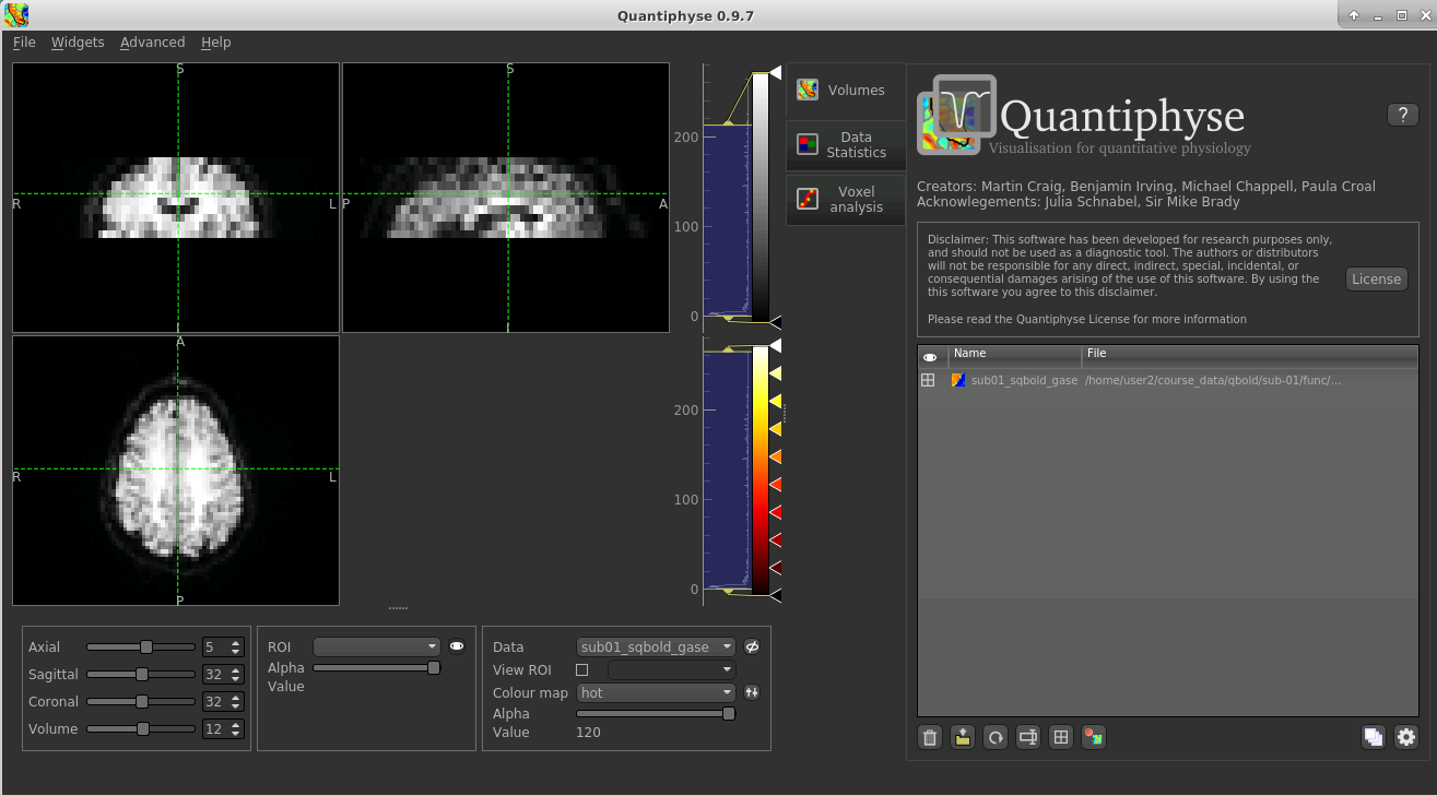
Image view
The left part of the window normally contains three orthogonal views of your data. In this case the data is a 2D slice so Quantiphyse has maximised the relevant viewing window. If you double click on the view it returns to the standard of three orthogonal views - this can be used with 3D data to look at just one of the slice windows at a time.
- Left mouse click to select a point of focus using the crosshairs
- Left mouse click and drag to pan the view
- Right mouse click and drag to zoom
- Mouse wheel to move through the slices
- Double click to ‘maximise’ a view, or to return to the triple view from the maximised view.
Widgets
The right hand side of the window contains ‘widgets’ - tools for analysing and processing data. Three are visible at startup:
Volumesprovides an overview of the data sets you have loadedData statisticsdisplays summary statistics for data setVoxel analysisdisplays timeseries and overlay data at the point of focus
Select a widget by clicking on its tab, just to the right of the image viewer.
More widgets can be found in the Widgets menu at the top of the window. The tutorial
will tell you when you need to open a new widget.
For a slightly more detailed introduction, see the Getting Started section of the User Guide.
Pre-processing
Slice Averaging
The GESEPI ASE pulse sequence mitigates the effect of magnetic field inhomogeneity by phase
encoding each 5 mm slice into four 1.25 mm sub-slices. To improve SNR these sub-slices are
averaged together. So in the case of the data we are analysing here, the original 40 slices
are reduced to 10 slices. Due to a 2.5 mm slice gap between the slices the NIFTI header reports
the slice thickness as 7.5 mm. The data suppplied in course data has already had slice
averaging performed.
Note
To perform slice averaging on the raw data you can use a command line script zaverage.sh,
for example: zaverage.sh sub-01_task-csfnull_rec-filtered_ase sub-01_sqbold_gase
Brain Extraction
For clinical data, we recommend brain extraction is performed as a preliminary step using FSL’s BET tool [6], with the
–m option set to create a binary mask and the -Z option to improve the brain extraction due to the small number of slices.
Using a brain ROI is strongly recommended as this will decrease processing time considerably.
In this case we will perform brain extraction from within Quantiphyse. We do not currently support the -Z option so
we will adjust the threshold to get a reasonable result.
Before brain extraction we will need to take the mean of the 4D data as Bet can only run on a 3D image. To do this we can use the
Processing->Simple Maths widget which allows us to do simple operations on data sets, similar to FSL maths. Select the
4D qBOLD data and enter the following expression:
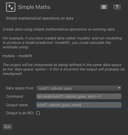
If you know Python and Numpy you will recognize this code - we can use any simple Numpy expression in the widget.
Now, from the Widgets menu select FSL->BET and then as input data choose the mean data we have just generated.
Check the Output brain mask option so we get a binary ROI mask for the brain and change the intensity threshold value to 0.4.
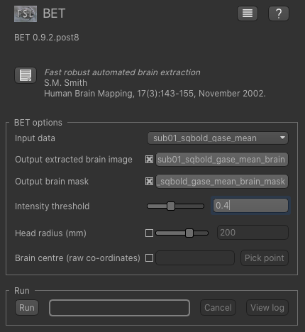
Click Run and an ROI should be generated covering the brain and displayed as follows:
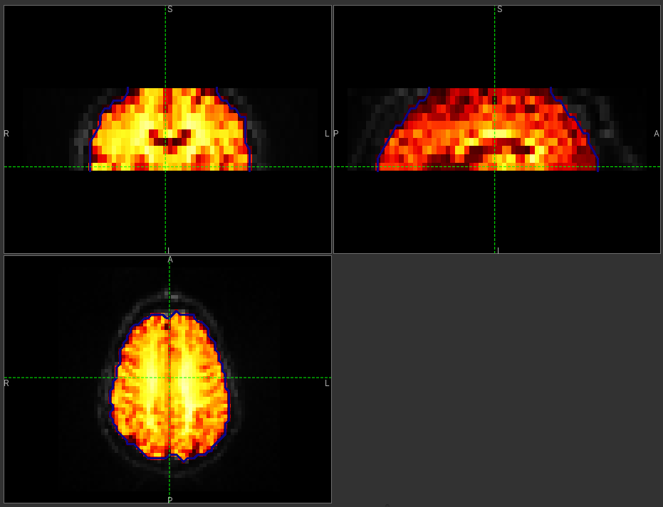
When viewing the output of modelling, it may be clearer if the ROI is displayed as an outline, as shown in this screenshot, rather than a shaded region. To do this, click on the icon to the right of the ROI selector (below the image view):
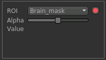
The icon cycles between display modes for the ROI: shaded (with variable transparency selected by the slider below), shaded and outlined, just outlined, or no display at all.
Note
It is possible to generate the brain mask from within Quantiphyse using the FSL integration plugin. We have not done this because the plugin does not currently support the -Z option and because it is necessary to take a the mean of the qBOLD timeseries before performing brain extraction
Note
If you accidentally load an ROI data set as Data, you can set it to be an ROI using the Volumes widget
(visible by default). Just click on the data set in the list and click the Toggle ROI button.
Motion Correction
Motion correction can be implemented using FSL’s MCFLIRT tool within Quantiphyse, or beforehand using FSL or another
tool. To run within Quantiphyse, select Widgets -> Registration -> Registration.
To run motion correction on the data, you need to:
- Set the registration mode to
Motion Correction- Ensure the method is set to
FLIRT/MCFLIRT- Select
sub-01_sqbold_gaseas theMoving data- Select the reference volume as
Specified volume- For GESEPI ASE data we’ll use the spin echo (tau=0) image, which in this case is image 7, so we have set
Index of reference volumeto 7- The output name can be left as the default:
sub-01_sqbold_gase_reg
The resulting setup should look like this:
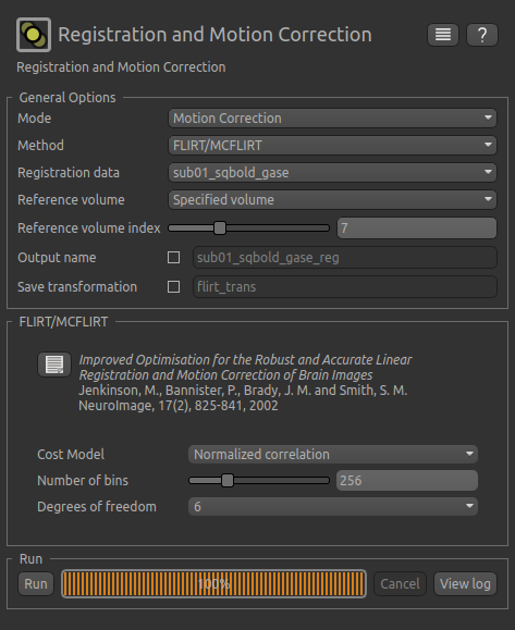
Click Run to run the motion correction. The output in this case is not very different from the input - you may be
able to see some small differences, by switching between sub-01_sqbold_gase and sub-01_sqbold_gase_reg in the
verlay selector (below the image view). You can also see differences using the Voxel Analysis widget - see below.
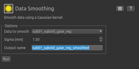
Data Smoothing
To suppress isolated noisy voxels we perform sub-voxel smoothing using the widget built in to Quantiphyse.
From the menu select Widgets->Processing->Smoothing and set the options to smooth sub-01_sqbold_gase_reg with
a smoothing kernel of 1.5 mm. This value is equivalent to smoothing with a full width half maximum equal to
the in-plane voxel dimension of 3.75 mm (FWHM ≈ 2.355 σ).
Visualising Data
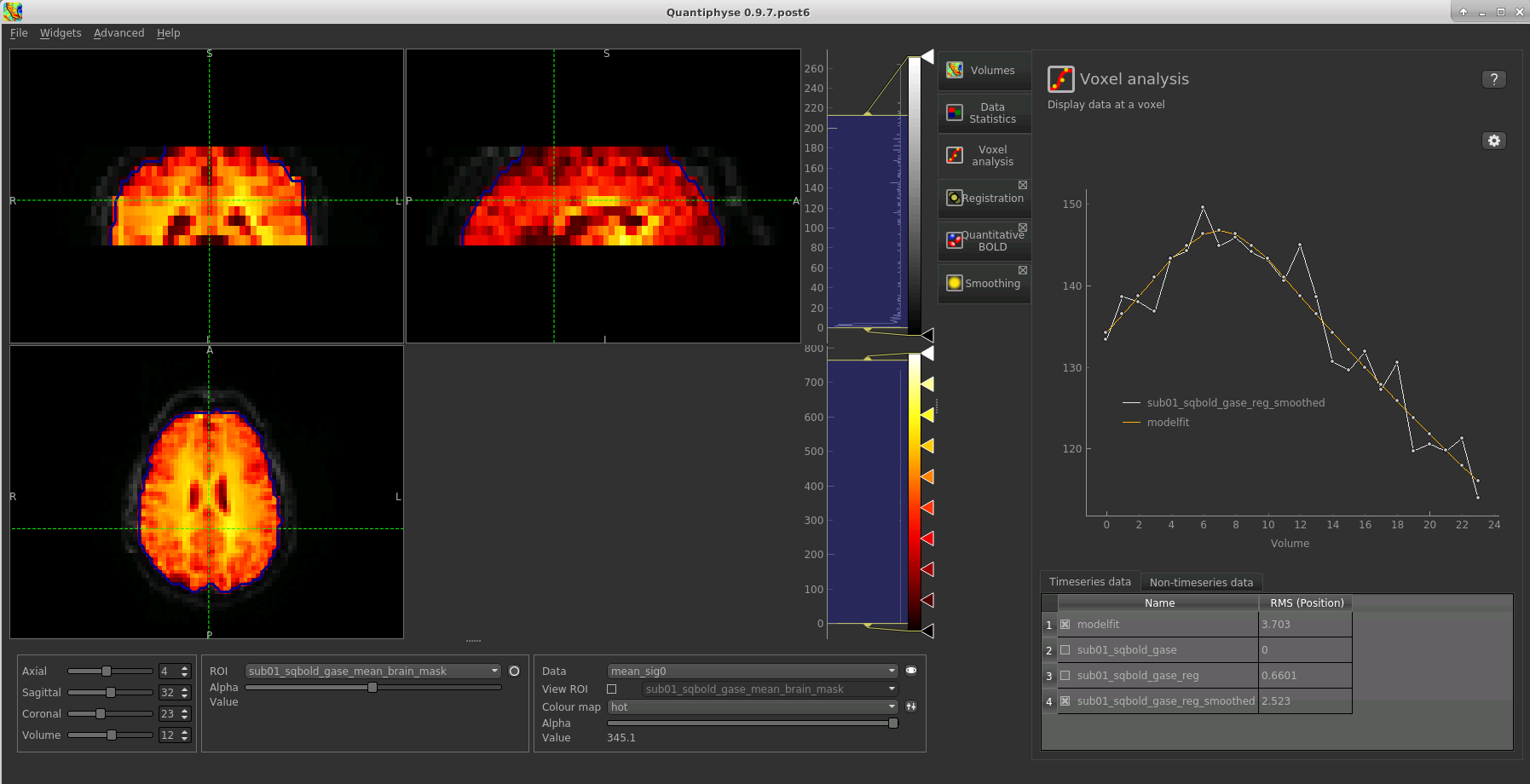
Select the Voxel Analysis widget which is visible by default to the right of the viewing window. Try clicking
on different voxels in the cortical grey matter to see the qBOLD signal curve:
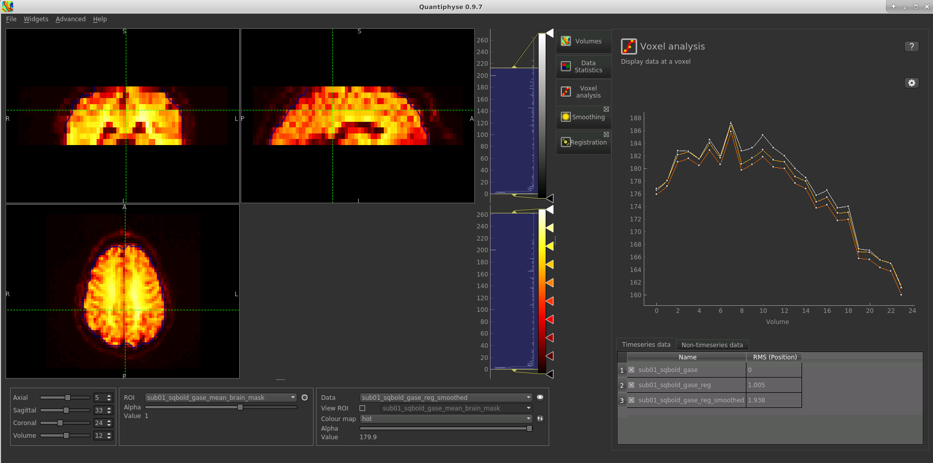
You can see the relatively subtle effect the motion correction and smoothing have had on the data. The checkboxes
in the Timeseries Data list can be used to show and hide data sets from the timeseries plot.
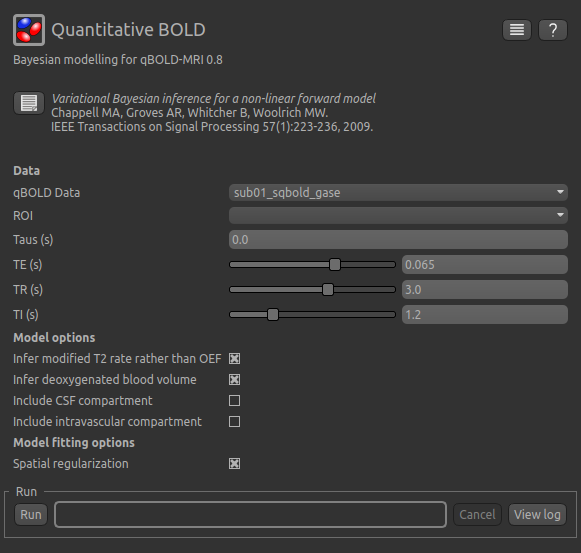
Bayesian Model-based Analysis
To analyse qBOLD data using Bayesian model fitting, select the Quantitative BOLD tool from the menu:
Widgets->BOLD MRI->Quantitative BOLD. The widget should look something like this:
Data and sequence section
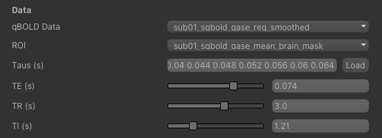
To begin with, make sure the sub-01_sqbold_gase_reg_smoothed data set is selected as the qBOLD data,
and the sub-01_sqbold_gase_mean_brain_mask brain mask is selected as the ROI.
Next we will specify the spin echo displacement times, or Taus - they represent the different \(R_2^\prime\) weightings acquired in the data set. You can enter them manually, or if they are stored in a text file (e.g. with one value per row) you can drag and drop the file onto the entry widget.
For this tutorial we have provided the Tau values in the file tau_values.txt which is in the sub-01 folder,
so click Load, select this file and verify that the values are as shown in the screenshot below.
Now set the echo time (TE) of the acquired data - in this case it is 0.074 s - and the repetition time (TR) - which is 3 s. In order to remove the confounding effect of CSF a FLAIR preparation is used to null the CSF signal. This value is set based on the TR and the T1 of CSF (3817 ms), which gives an inversion time (TI) of 1210 ms, or 1.21s.
The sequence parameters should appear as follows:
Model Options
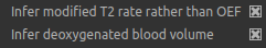
The default options are Infer modified T2 rate rather than OEF and Infer deoxygenated blood volume. The latter
ensures that DBV is mapped on a voxel by voxel basis rather than using a fixed value and the former causes the model
to estimate \(R_2^\prime\) and DBV rather than OEF and DBV. This is an important point in the fitting of qBOLD data.
It has been shown that OEF and DBV are relatively colinear in the parameter space meaning that a unique solution is
difficult to find [1], [7]. In contrast, \(R_2^\prime\) and DBV have much lower correlation providing the
opportunity to accurately estimate both simultaneously.
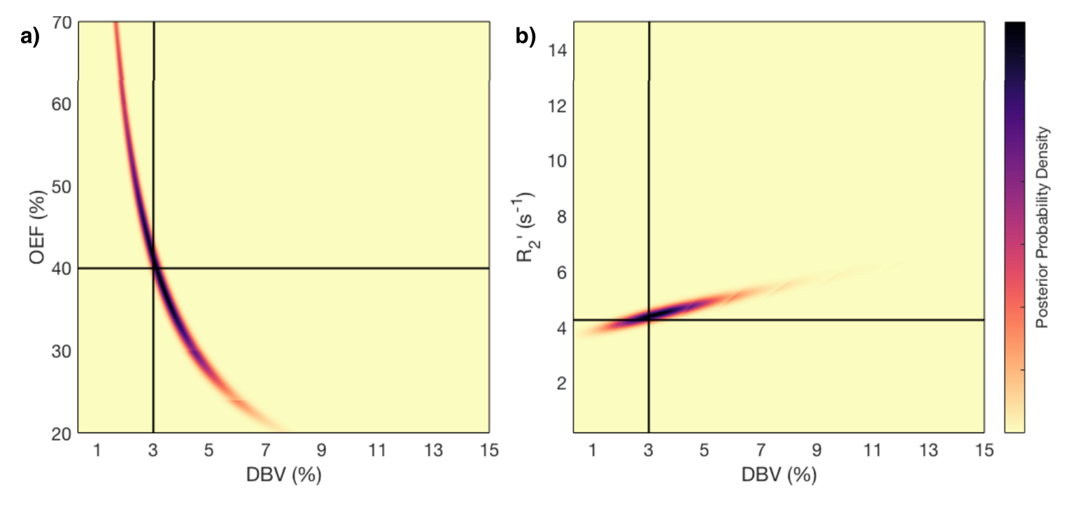
M. T. Cherukara, A. J. Stone, M. A. Chappell, and N. P. Blockley, “Model-Based Bayesian Inference of Brain Oxygenation Using Quantitative BOLD” Neuroimage, In Press, 2019. doi: 10.1016/j.neuroimage.2019.116106. Published by Elsevier and licensed under CC BY 4.0.
This figure shows the results of a grid-search posterior sampling on simulated ASE qBOLD data. (a) shows the posterior probability of OEF-DBV parameter pairs with the true values shown by the black cross-hair. (b) show the posterior probability of R2′-DBV pairs using the same simulated data. In the OEF-DBV model, there is a large area of collinearity, and the posterior density distribution does not have a Gaussian-like form. By contrast, the R2′-DBV model has more separable parameters, and a distribution shape that can more easily be approximated by a multivariate normal distribution, which is a requirement for the variational Bayes inference methods used by this tool.
When data does not include a FLAIR preparation to null CSF, Include CSF compartment can be checked. In this case you
will be presented with further options to Infer the CSF frequency shift and Infer CSF fractional volume.
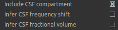
Since there is very little information regarding CSF in the GESEPI ASE data we are using, care should be taken when using these options
and it is likely that using a fixed value of frequency shift (unchecking Infer the CSF frequency shift) would be the most
likely option. If you would like to experiment with these options the data set linked above also includes GESEPI ASE data
without FLAIR (sub-01_task-nonull_rec-filtered_ase).
Finally, the qBOLD model was derived to account only for extravascular signal. It is possible to add a second intravascular
compartment to the analysis by checking Include intravascular compartment.
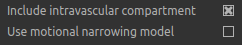
The standard model utilises the powder model used in the original qBOLD paper [5]. An alternative is the motional narrowing model which utilises an alternative model of the intravascular signal [8]. In general, the intravascular signal has a weak effect on the final results, but may be valuable in regions of the brain with intermediate DBV fractions i.e. not very high or very low.
Model fitting options
By default, Spatial regularization is selected. This will reduce the appearance of noise in the final parameter maps using
adaptive smoothing within the Bayesian framework in which the information present in the signal determines the degree of
spatial smoothing. Fine detail in the output is only preserved if the information in the data justifies it.
Running the analysis
The Run button is used to start the analysis. The output data will be loaded into Quantiphyse as the following data sets:
mean_r2p- Mean value of \(R_2^\prime\) predicted by the Bayesian modellingmean_dbv- Mean value of DBV predicted by the Bayesian modellingmean_sig0- Mean offset signal predicted by the Bayesian modellingmodelfit- Predicted signal timeseries for comparison with the actual data
Visualising Processed Data
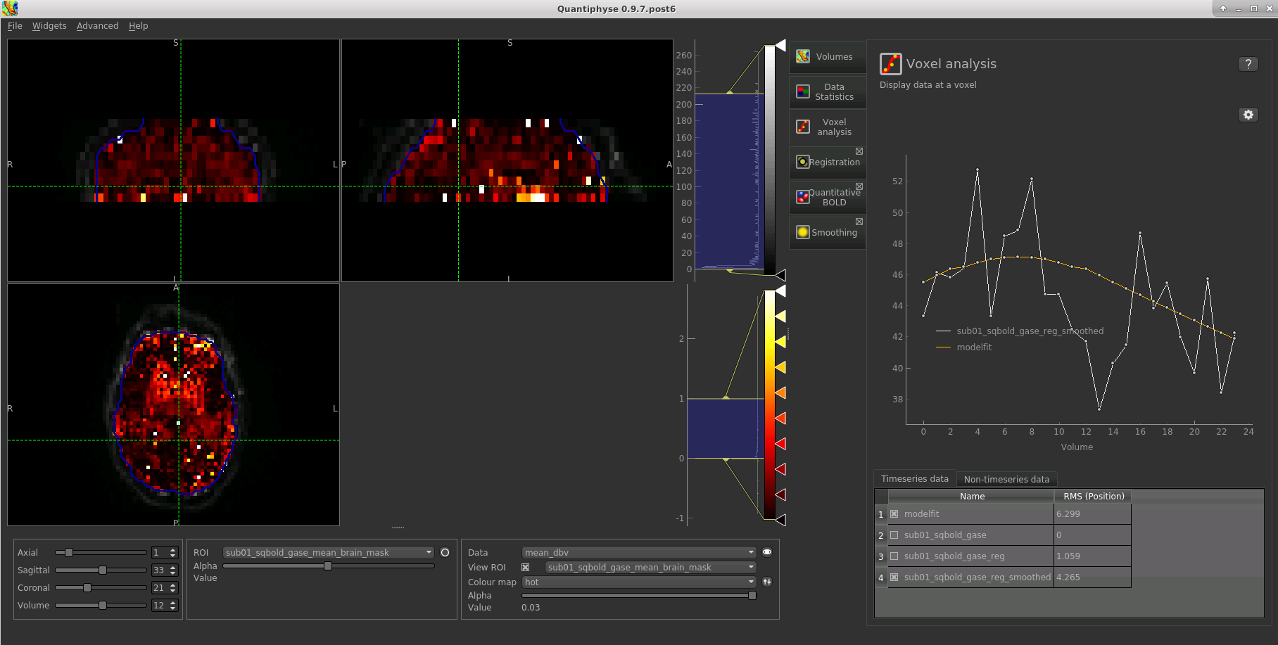
If you re-select the Voxel analysis widget which we used at the start to look at the qBOLD signal in the
input data, you can see the model prediction overlaid onto the data. By clicking on different voxels you
can get an idea of how well the model has fitted your data.
Parameter map values at the selected voxel are also displayed in Voxel Analysis. The various parameter maps can be selected for viewing from the Volumes widget, or using the overlay selector below the image viewer. This is the DBV output for this data:
To make this map visualisation clearer we have set the colour map range to 0-1 by clicking on the levels button  in the view options section, below the main viewer window. We have also selected the brain mask as the ‘View ROI’ which
means that the map is only displayed inside this ROI.
in the view options section, below the main viewer window. We have also selected the brain mask as the ‘View ROI’ which
means that the map is only displayed inside this ROI.
Estimating OEF when R2′-DBV has been performed
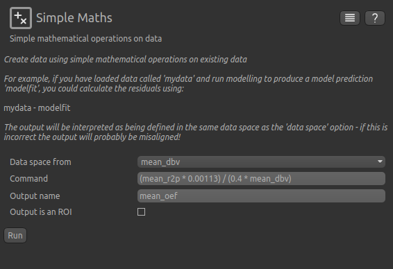
Our default recommendation is to fit \(R_2^\prime\) and DBV to the qBOLD data. Therefore, OEF is not an output of the model fitting procedure. Currently the maps of R2′ and DBV must be combined with tools such as fslmaths and the following equation:
\(OEF= \frac{3 \cdot R_2^\prime}{4\pi \cdot \gamma B_0 \cdot \Delta_{\chi_0} \cdot Hct \cdot DBV}\)
where \(\gamma = 267.5 \times 10^6 \text{rad} s^{-1} T^{-1}`\), \(B_0 = 3 T\), \(\Delta_{\chi_0} = 0.264 \text{ppm}\), and Hct is typically assumed to be 0.4. By combing these constants into a single constant \(c = 1.13 \times 10^{-3}\), we can simplify this equation to:
\(OEF=\frac{c \cdot R_2^\prime}{Hct \cdot DBV}\)
You can perform this conversion in Quantiphyse using Widgets->Processing->Simple Maths as follows:
Equivalently, this can be done using fslmaths as:
fslmaths r2p-map -div dbv-map -mul 0.00113 -div 0.4 oef-map
Note
fslmaths outputs zero for voxels outside the mask where there is a division by zero
whereas Quantiphyse will output a nan value here. To avoid this in quantiphyse you
can instead use the expression np.nan_to_num((mean_r2p * 0.00113) / (0.4 * mean_dbv))
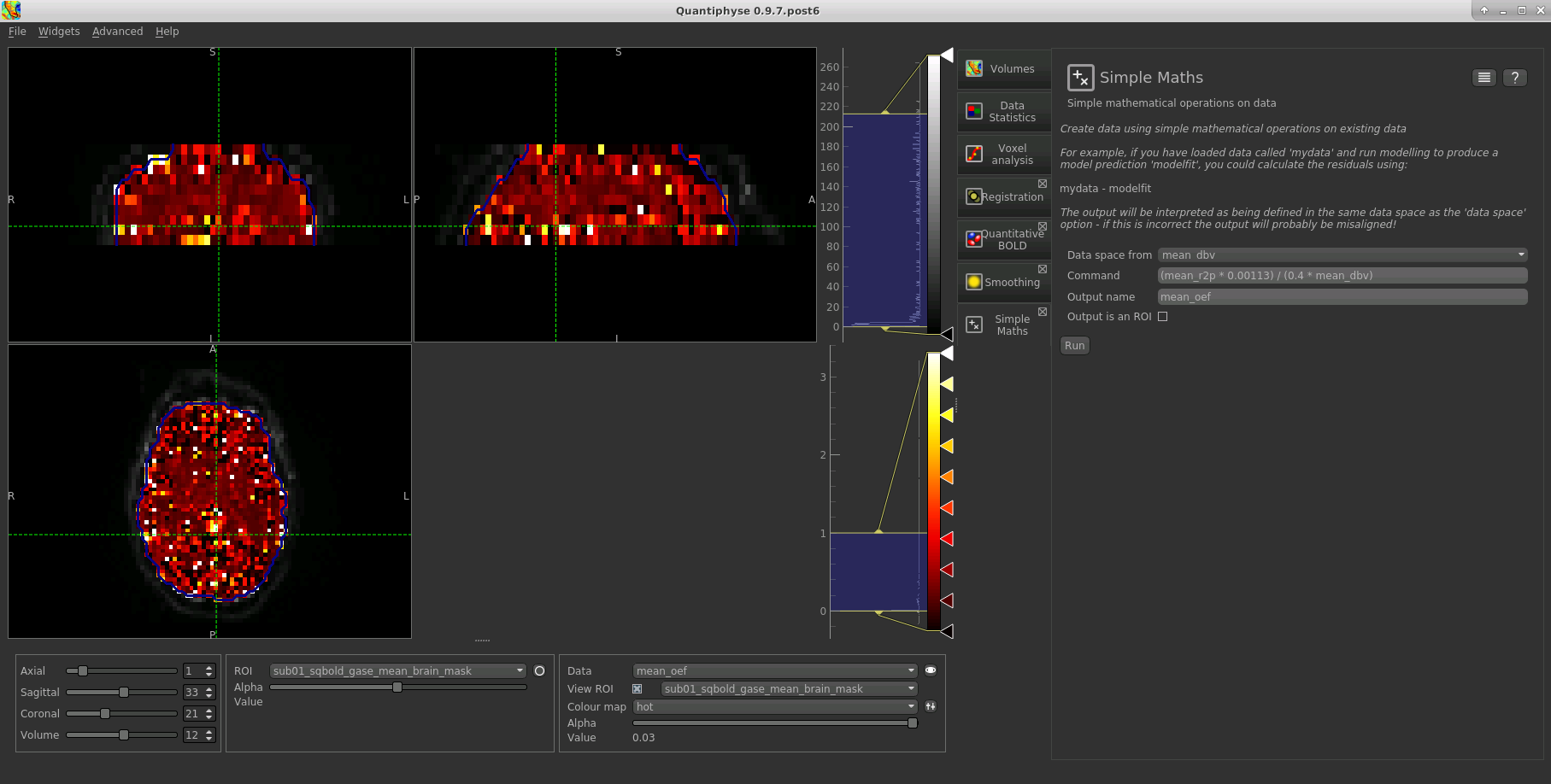
The OEF map for this data appears as follows, again using a colormap range of 0-1 and displaying in the ROI only:
References
| [1] | (1, 2)
|
| [2] |
|
| [3] |
|
| [4] |
|
| [5] | (1, 2)
|
| [6] |
|
| [7] |
|
| [8] |
|