QuantiCEST
- Widgets -> CEST -> QuantiCEST
This widget provides CEST analysis using the Fabber Bayesian model fitting framework.
To do CEST analysis you will need to know the following:
- The frequencies in the z-spectrum you sampled at. The number of frequencies corresponds to the number of volumes in your data
- The field strength - default pool data is provided for 3T and 9.4T, but you can specify a custom value provided you provide the relevant pool data
- The saturation field strength in µT
- For continuous saturation, the duration in seconds
- For pulsed saturation details of the pulse magnitudes and durations for each pulse segment, and the number of pulse repeats
- What pools you want to include in your analysis
- If default data is not available for your pools at your field strength, you will need the ppm offset of each pool, its exchange rate with water and T1/T2 values
Setting the sampling frequencies
The frequencies are listed horizontally:

You can type in your frequencies manually - the list will automatically grow as you add numbers.
However, you may have your frequencies listed in an existing text file - for example the dataspec file if you have been using Fabber
for your analysis. To use this, either drag the file onto the list or click the Load button and select the file. Quantiphyse will
assume the file contains ASCII numeric data in list or matrix form and will display the data found.
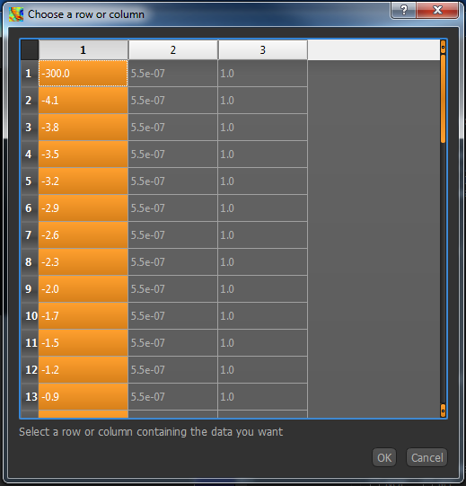
Click on the column or row headers to select the column/row your frequencies are listed in. In this case, we have a Fabber dataspec
file and the frequencies are in the first column, so I have selected the first column of numbers. Click OK to enter this into your
frequency list.

Setting the field strengths
Choose the B0 field strength from the menu. If none of the values are correct, select Custom and enter your field strength in the
spin box that appears

Note that you are being warned that the default pool data will not be correct for a custom field strength and you will need to edit them.
The saturation field strength is set using the B1 (µT) spin box below.
Continuous saturation
Select Continuous Saturation from the menu, and enter the duration in seconds in the spin box

Pulsed saturation
Select Pulsed Saturation from the menu.
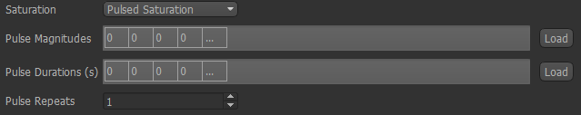
The pulse magnitudes and durations can be set in the same way as the sampling frequencies, so if you have them in a text file
(for example a Fabber ptrain file), drag it onto the list and choose the appropriate row/column.
The number of magnitudes must match the number of durations! Repeats can be set in the spin box at the bottom.
Choosing pools
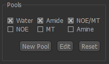
Six built-in pools are provided, with data at 3T and 9.4T, you can choose which to include using the checkboxes.
Each pool is characterized by four parameters:
- The ppm offset relative to water (by definition this is zero for water)
- The exchange rate with water
- The T1 value at the specified field strength
- The T2 value at the specified field strength
To view or change these values, click the Edit button.
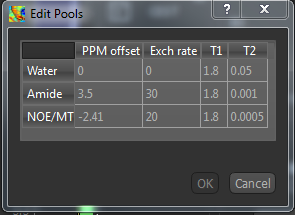
A warning will appear if you change the values from the defaults. Obviously
this will be necessary if you are using a custom field strength. If you want to return to the original values at any point, click the
Reset button. This does not affect what pools you have selected and will not remove custom pools
Custom pools
If you want to use a pool which is not built-in, you can use the New Pool button to add it. You will need to provide the four parameters above, and your new pool will then be selected by default.
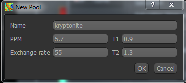
Warning
Currently custom pools, and custom pool values are not saved when you exit Quantiphyse
Analysis options
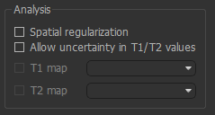
These affect how Fabber performs the model fitting
Spatial regularization- if enabled, adaptive smoothing will be performed on the parameter maps, with the degree of smoothing determined by the variation of the dataAllow uncertainty in T1/T2 values- T1/T2 will be inferred, using the pool-specified values as initial priorsT1 map/T2 map- If inferring T1/T2, an alternative to using the pool-specified values as priors you may provide existing T1/T2 maps for the water pool.
Warning
Spatial regularization prevents Fabber from processing voxels in parallel, hence the analysis will be much slower on multi-core systems.
Run model-based analysis
This will perform the model fitting process.
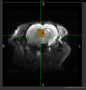
CEST analysis is computationally expensive, and it is recommended to run on a small ROI before attempting your full data set. The ROI Builder tool is an easy way to define a small group of voxels to act as a test ROI, e.g. as below
The output of the model-based analysis is a set of data overlays as follows:
mean_B1_off- Model-inferred correction to the specified B1 valuemean_ppm_off- Model-inferred correction to the ppm values in the z-spectrum.modelfit- Model z-spectrum prediction, for comparison with raw datamean_M0_Water- Inferred magnetization of the water poolmean_M0_Amine_r,mean_M0_NOE_r, ..etc - Inferred magnetization of the other pools, relative to M0_Watermean_exch_Amine,mean_exch_NOE, ..etc - Inferred exchange rates of non-water pools with watermean_ppm_Amine,mean_ppm_NOE, ..etc - Inferred ppm frequencies of non-water poolscest_rstar_Amine,cest_rstar_NOE, ..etc - Calculation of R* for non-water pools - see below for method
If T1/T2 values are being inferred (Allow uncertainty in T1/T2 values is checked), there will be additional outputs:
mean_T1_Water,mean_T1_Amine, ..etc - Inferred T1 values for each poolmean_T2_Water,mean_T2_Amine, ..etc - Inferred T2 values for each pool
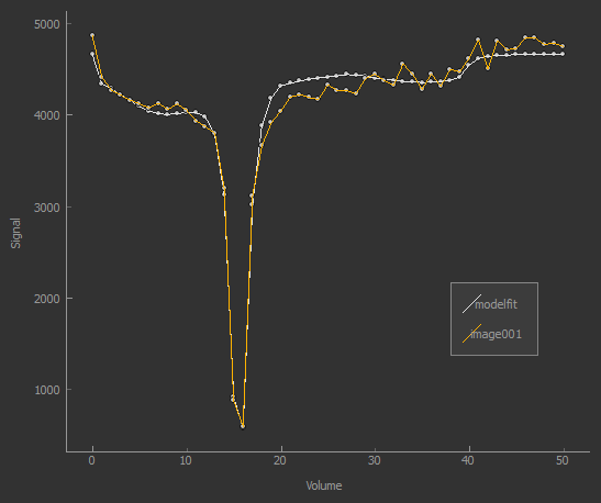
The screenshot below (from the Voxel Analysis widget) shows the model fitting to the z-spectrum.
CEST R* calculation
The R* calculation is performed as follows:
- After the model fitting process, for each non-water pool, two separate z-spectrum predictions are evaluated at each voxel: - The spectrum based on the water pool only - The spectrum based on the water pool and each other pool individually
- The parameters used for this evaluation are those that resulted from the fitting process, except that: - T1 and T2 are given their prior values - The water ppm offset is zero
- Each spectrum is evaluated at the pool ppm resonance value and the normalized difference to water is returned:
Lorentzian difference analysis
This is a quicker alternative to model-based analysis, however less information is returned.
The calculation is performed using the Fabber fitting tool as previously, in the following way:
- Only the water pool is included, i.e. just fitting a single Lorentzian function to the z-spectrum
- Only data points close to the water peak and unsaturated points are included. Currently this means points with ppm between -1 and 1 are included as are points with ppm > 30 or <-30
- The raw data is subtracted from the resulting model prediction at all sampled z-spectrum points
The output of the LDA calculation is provided as a multi-volume overlay lorenz_diff.