ASL Analysis
- Widgets -> ASL -> Model fitting
This widget provides Arterial Spin Labelling MRI analysis using the Fabber Bayesian model fitting framework.
ASL data structure
To do ASL model fitting you will need to define the structure of your ASL data, using the ASL structure widget
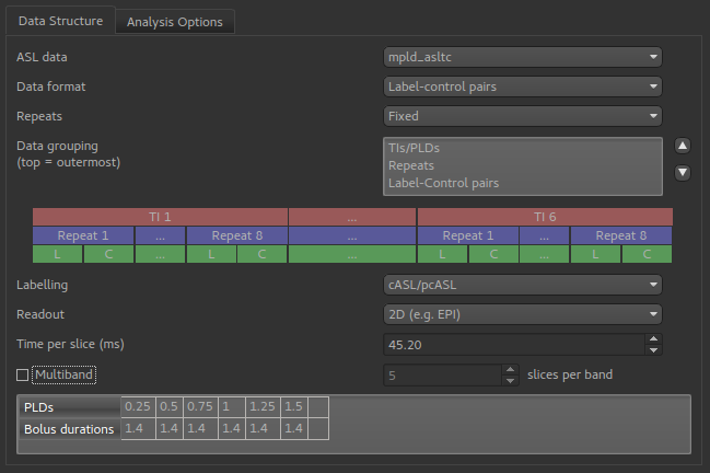
This example shows a multi-PLD PCASL data set with 2D readout.
Model fitting options
In addition, a number of options may be specified for the model fitting process on the Analysis tab.
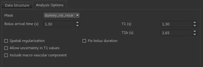
Bolus arrival timeis an estimate - with multi-PLD data it’s actual value will be estimated based on the data.T1andT1bare estimated T1 values for tissue and blood. By default these are fixed, however theAllow uncertainty in T1 valuesoption will cause them to be estimated from the data, using the specified values as Bayesian priors.Spatial regularizationwill smooth the data using an adaptive method which depends on the degree of variation in the data.Include macro vascular componentwill allow an additional arterial component in the fitting process.Fix bolus durationNormally the bolus duration is allowed some variation to better fit the data. Selecting this option will fix it to the user specified value.
Warning
Spatial regularization prevents Fabber from processing voxels in parallel, hence this part of the analysis will be much slower that the other steps on multi-core systems.
Click Run to start the analysis. Typically the analysis occurs in multiple stages which are displayed in the Run ASL modelling
box. Note that the final spatial step does not currently give progress updates, so it may appear to have hung while this is running.
Output data
The following data items are returned:
perfusionTissue perfusiondurationBolus duration, unless this is fixedarrivalInferred bolus arrival timemodelfitModel prediction for comparison with the tag-control differenced data
If Include macro vascular component is specified:
aCBV
If Allow uncertainty in T1 values is specified:
mean_T_1Tissue T1 valuemean_T_1bBlood T1 value
For each of these data items, a standard deviation map will also be produced with the suffix _std. This reflects the output
of the Bayesian inference - the value of a parameter at a given voxel is represented as a Gaussian probability distribution with
a mean value (the parameter map) and a standard deviation (_std map).
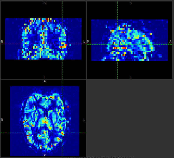
An example perfusion map without spatial regularization might look like this:
With spatial regularization turned on, the same data set produced the following perfusion map:
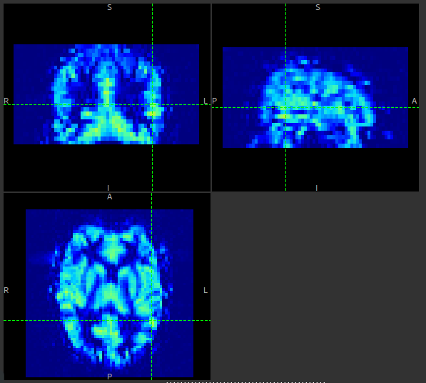
The effect is similar to what you would get by applying a smoothing algorithm to the output, however in this case the degree of smoothing is determined by the the variation in the data itself.